Data Structures for Large-Scale Systems

Probabilistic Data Structures: Bloom filters, Count-min sketch, and HyperLogLog

Imagine you’ve just deployed a new microservice, a simple API gateway, and initially, traffic is pretty manageable, maybe a few requests per second. And you’re logging every IP address to track unique visitors and block malicious spammers.

For the first week, everything is smooth. Your monitoring dashboard is green. You’re using a standard Set or HashMap in memory to store these IP addresses. It’s exact, it’s fast, and the code is clean.

But then, the product goes viral, or maybe, a massive client onboards, and your user base increases exponentially. Suddenly, you aren’t dealing with 1,000 or 10,000 requests. You’re dealing with 100 million events a day.

This is where the naive approach of using a traditional data structure hits a wall.

The Memory Wall

Here is the thought process that usually follows. You look at the metrics and realise your memory usage is spiking.

Why? Because exactness is expensive.

If you are storing 100 million IPv6 addresses in a HashMap, you aren’t just storing the data, you’re storing the overhead of the data structure itself. Overhead here refers to the extra memory required by the data structure, i.e., pointers, metadata, unused capacity, object wrappers and not the IPv6 addresses themselves.

An IPv6 address is only 16 bytes. In theory, 100 million of them should fit in about 1.6 GB. In practice, a HashMap stores far more than that: per-entry objects, references, hash tables, and unused capacity. That overhead is what pushes memory usage into the multi-gigabyte range. We are talking gigabytes of RAM just to answer a simple question: “How many times have we seen this user before?”

In the cloud world, memory is money, and burning through gigabytes of memory just for a counter isn’t good engineering, it’s inefficiency.

And it gets worse. What if you need to do this across a distributed system? Do you replicate that massive HashMap across every node? The network latency alone will kill your throughput.

We need a better strategy. We need to trade a tiny bit of accuracy for a massive gain in efficiency.

Enter Probabilistic Data Structures

This is where we make the tradeoff. We use algorithms with data structures that use a fraction of the memory, often KBs instead of GBs, by accepting a known error rate.

Probabilistic data structures take a different approach. Instead of storing every item exactly, they rely on hashing and controlled uncertainty to dramatically reduce memory usage. They’re commonly used for problems like membership checks, frequency counting, and estimating how many unique elements you’ve seen. Each input is passed through one or more hash functions that map it to positions in a small underlying array, allowing many items to share the same space. The result isn’t perfectly accurate, but the error is known and bounded — and in exchange, you get massive savings in memory and performance at scale.

Let’s look at the three of them we typically see in production environments.

1. The Bloom Filter: Probably Yes, Definitely No

This first data structure is used to perform membership checks in large data sets.

Let’s say you want to check if a username is already taken during the signup process, or if a URL is malicious. You don’t need to store the whole string of the usernames that have already been seen by the server. Instead, you just store indicators to check whether the server has seen the incoming username.

The Bloom Filter provides the combination of the data structure and algorithm to be able to do so.

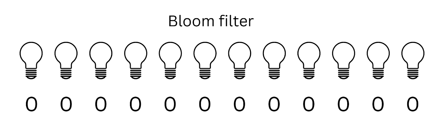
A Bloom Filter is like a row of light switches (bits), initially all set to ‘off’ (0).

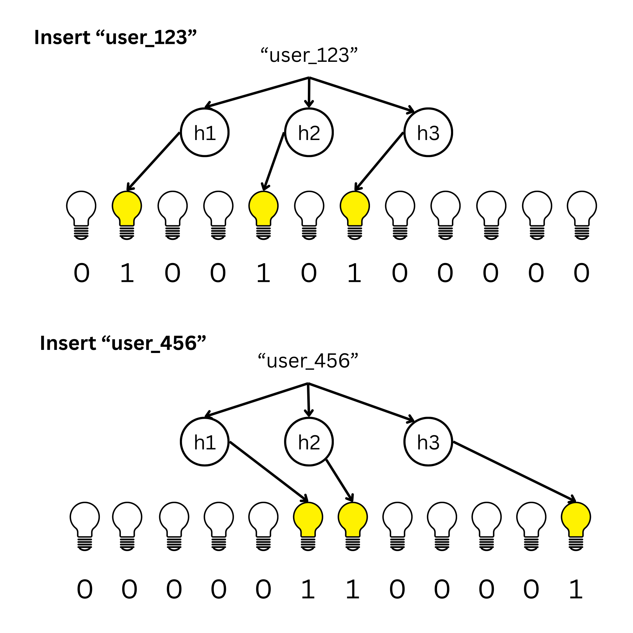
When a new item comes in, you run it through a few hash functions, each pointing to a position in the array. These functions tell you which switches to flip ‘on’ (1).

To check if an item exists, you hash it again. If all the corresponding switches are on, the item is probably there. If even one switch is off, the item is definitely not there.

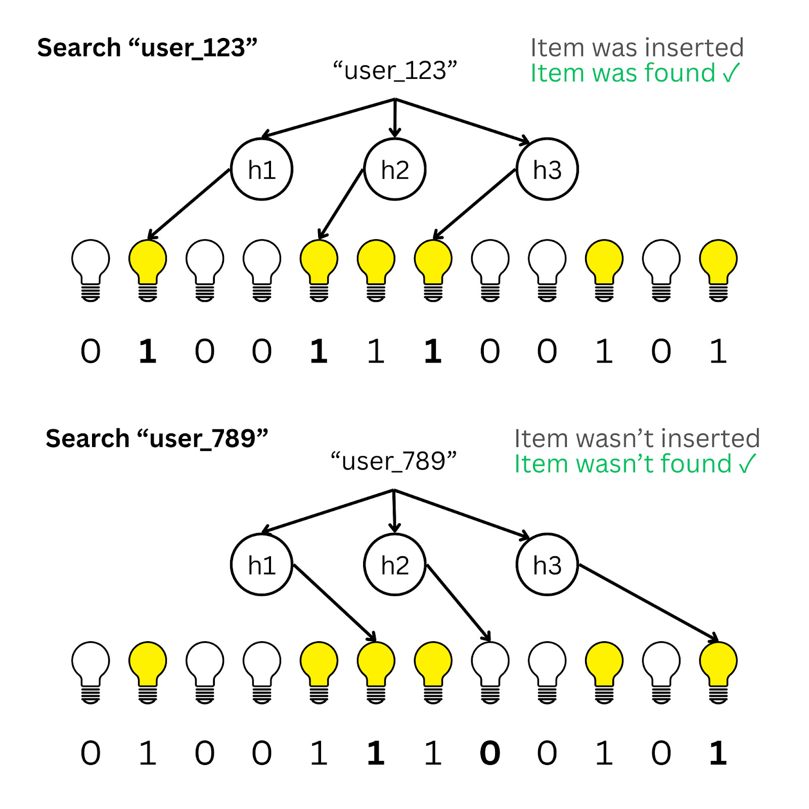
However, the hash functions can incorrectly map a queried item to positions that are set even when the item wasn’t inserted.

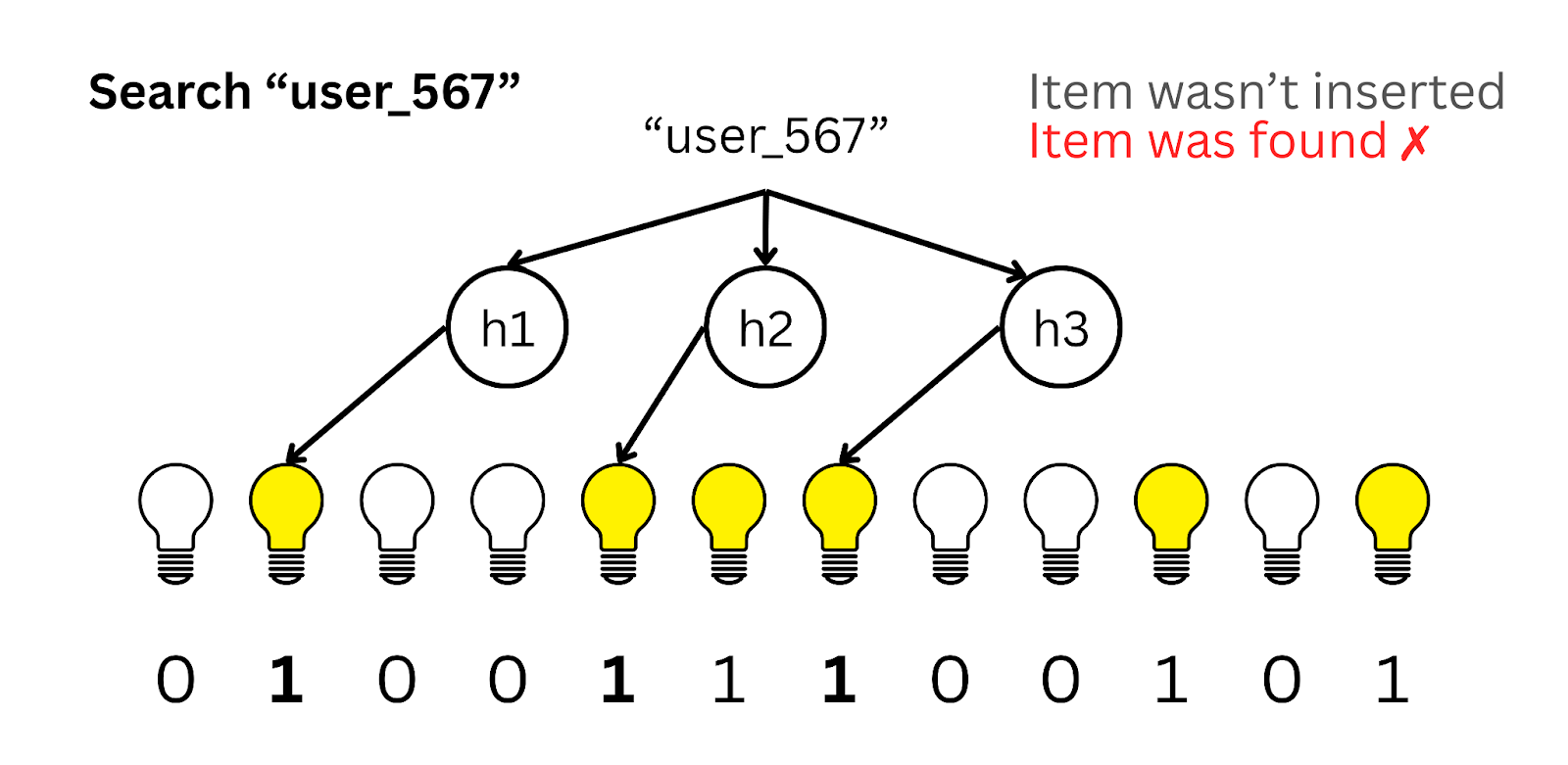
This leads to a False Positive. Thus, when all bits are set we can only say that the queried item may exist and cannot guarantee that it exists.

The Tradeoff

You might get a False Positive (it says yes, but it’s actually not true). But you will never get a False Negative. For a cache or a spam filter, that’s a trade I’m willing to take to save 90% of my RAM.

2. Count-Min Sketch: The Heavy Hitters

This data structure is used for counting the frequency of an item in a dataset.

Suppose you are analysing logs to find the ‘Top 10’ most frequent API consumers or the most popular products on a dashboard. You don’t care about the user who visited once, you care about the heavy hitters.

Storing a counter for every single ID is wasteful. Instead, we use a Count-Min Sketch.

Think of this as a 2D grid of counters, a matrix. When an event comes in, we hash it to map it to a specific cell in each row and increment those counters.

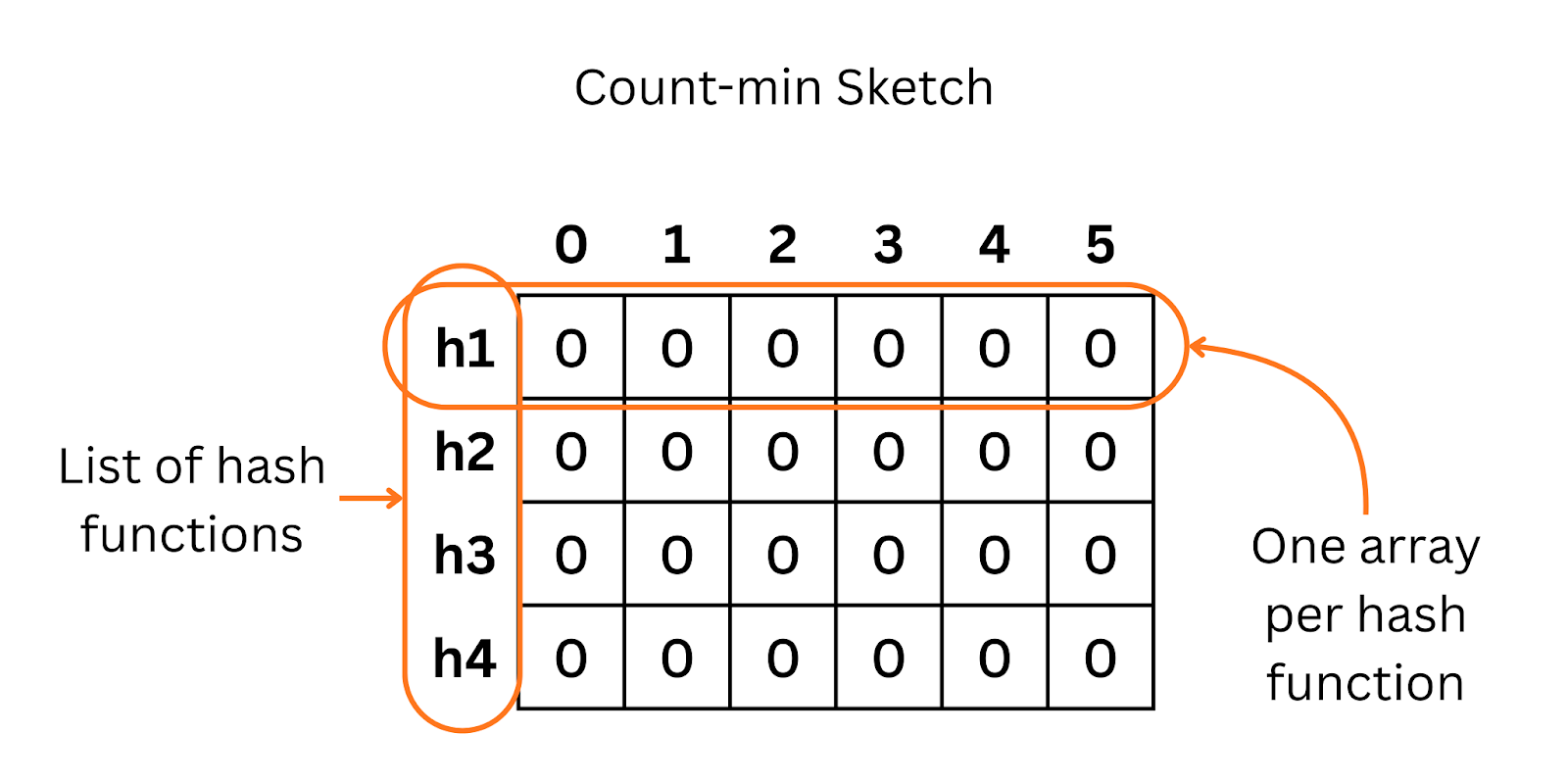
To get the frequency of an item, we look at all the cells it maps to and take the minimum value among them.

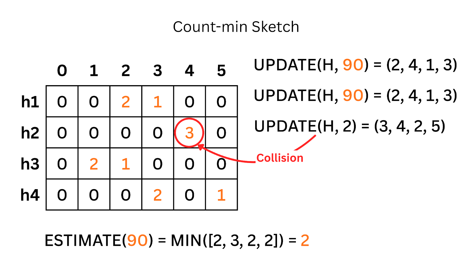
The Tradeoff

Because of collisions (different items mapping to the same cell), the count might be slightly higher than reality (overestimation). But it will never be lower. It lets us track trends in massive streams with constant space.

Thus, using Count-min Sketch, we can track frequent visitors, IPs producing unusual traffic, or any viral posts on scale without too much memory overhead.

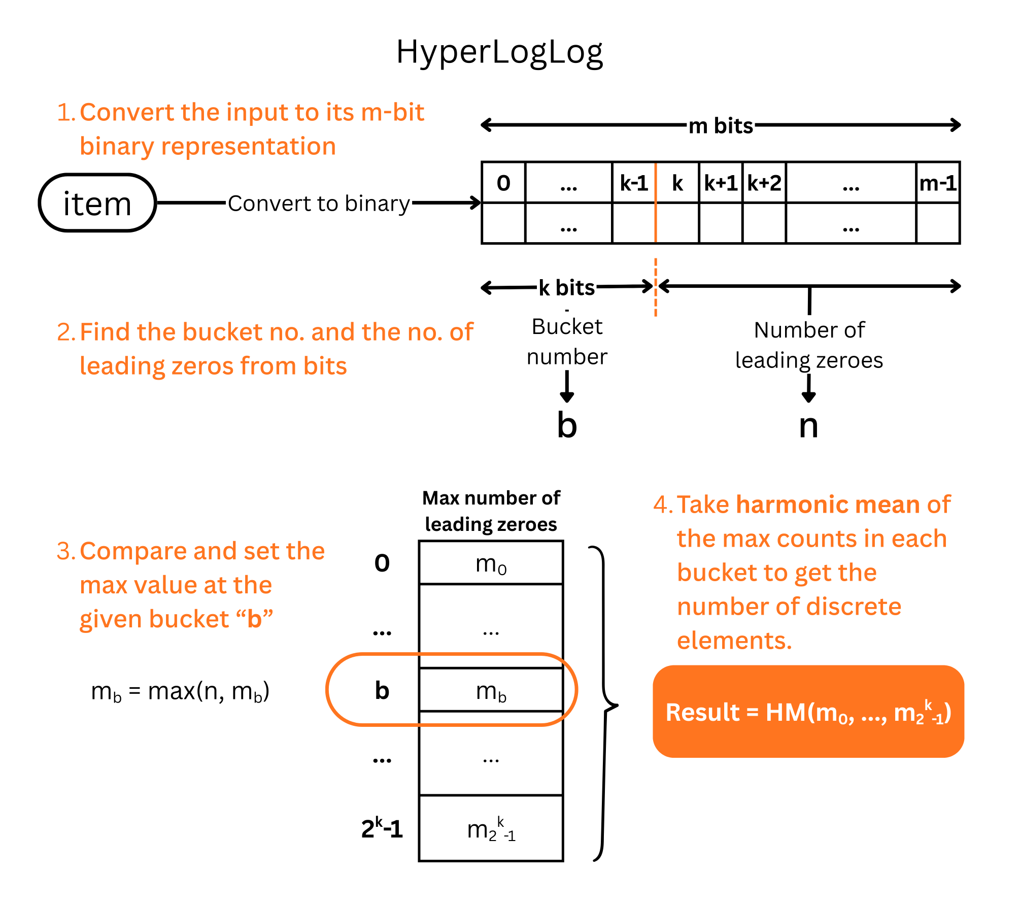
3. HyperLogLog: Counting the Crowd

This solves the classic analytics problem: ‘How many unique users visited the site today?’ (Cardinality).

If you have 1 billion events, storing all unique IDs to count them is a nightmare. HyperLogLog solves this by looking at the randomness of data.

It hashes the user ID and looks at the binary representation. Specifically, it looks for the longest run of leading zeros.

The intuition is simple: getting a hash that starts with 0000 is much rarer than a hash starting with 0. The longer the run of zeros, the more unique elements we have likely seen.

The Tradeoff

You don’t get an exact number like ‘1,047,367 users’. You get ‘approximately 1 million users with a 2% standard error’. For analytics and billing tiers, that is usually accurate enough, given the insane amount of memory saved.

Along with usages in analytics workloads, it can also be used in Database systems to estimate cardinality of a column, and then the queries can be written based on the cardinality.

That said, HyperLogLog should only be used if the dataset is too large, if not, there is no point and a simple hash set would be better for accuracy.

---

In high-throughput systems, approximate answers delivered instantly and cheaply are often worth more than exact answers that crash your pods.

Thus, we use these approximate data structures in the system rather than conventional exact data structures that grow unbounded.

In the upcoming posts, we are going to dive deep into each.

---