
Probabilistic Data Structures: The Bloom Filter Deep Dive


In the last post, we hit the Memory Wall. We realised that storing millions of exact keys in RAM isn’t just expensive, it’s a recipe for crashing your pods and burning money. We introduced the concept of Probabilistic Data Structures that trade a tiny bit of accuracy for a massive gain in efficiency.
Today, we are going to look under the hood of the most famous one: The Bloom Filter.
We often worry about how fast our database can find data. But we rarely ask the opposite question: How fast can our database say “I don’t know”?
As it turns out, saying “No” is surprisingly expensive. To confirm something doesn’t exist, a system usually has to scan indices or check the disk. The Bloom Filter is the mathematical in-memory shortcut. It’s like a bouncer that stands in front of your database and says, “Don’t bother checking inside. I can tell you right now, that guy isn’t here.“
This is why Apache Cassandra uses Bloom Filters per SSTable to avoid unnecessary disk reads. Google Bigtable does the same to protect its storage layer from pointless I/O. A few false positives are acceptable, but false negatives are not, so the correctness is maintained while the performance skyrockets.
Part 1: The Theory (Cats, Dogs, and Light Switches)
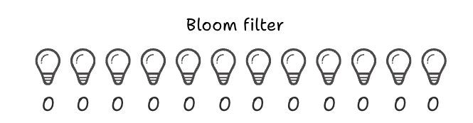
At its core, a bloom filter essentially is just a very long, empty array of bits(0s and 1s) that works together with a group of hash functions. No objects, pointers or any sort of overhead.
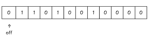
As mentioned in the previous blog, think of it as a massive row of Light Switches, all initially flipped ‘OFF’ (0).
Let’s say we are working with a Bloom Filter of 12 bits.
To make this work, we need hash functions. For example, let’s take 3 hash functions, the actual formula to calculate hash optimally is discussed later in the blog.
Act 1: Flipping the First Switches
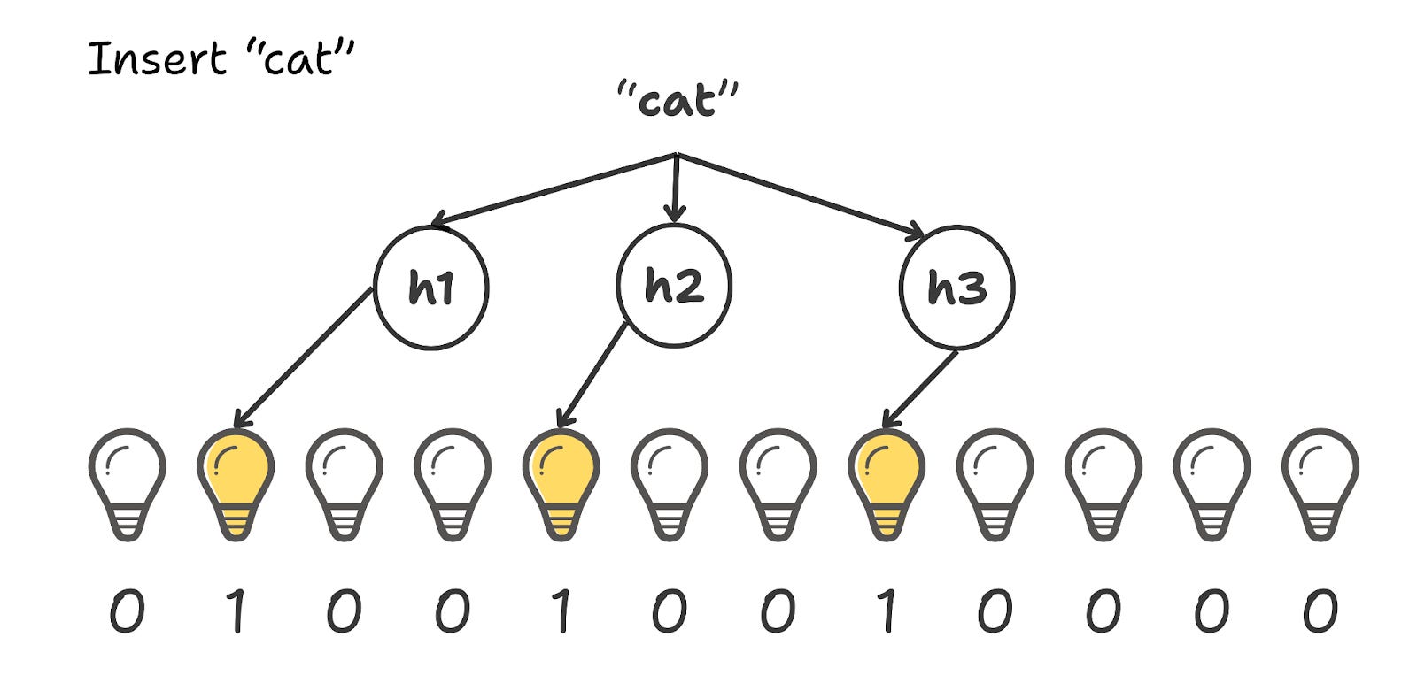
We want to add “cat” to the set. We run the string through our 3 hash functions.
Real hash functions output massive integers (like 2,148,901), but we only have 12 slots in our array. We can’t flip a switch that doesn’t exist. To fix this, we use the modulo operator (%), and mod the hash with the total number of bits we are using, so it is always in range.
In our case, it takes the huge number, divides it by 12, and gives us the remainder, guaranteeing the result always fits perfectly between 0 and 11.
h₁(”Cat”) → 2,148,901 % 12 = 1
h₂(”Cat”) → 8,392,012 % 12 = 4
h₃(”Cat”) → 5,000,011 % 12 = 7
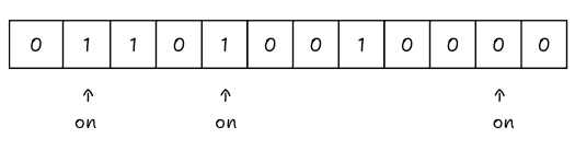
We go and flip those switches ON.
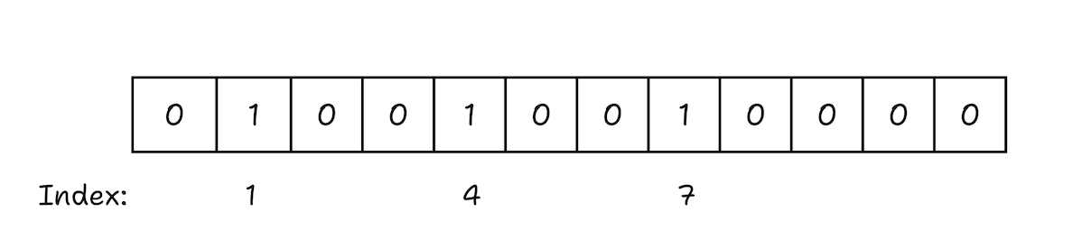
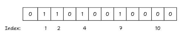
The array of bits, or rather our bloom filter now becomes
Act 2:The Shared Switch (dog)
Next, we add “dog”.
h₁(”Dog”) → 2
h₂(”Dog”) → 4
h₃(”Dog”) → 10
We go to the array to flip switches 2, 4, and 10.
Now, Switch 4 was already turned on by “Cat” in the previous step.
In a Bloom Filter, this is fine. We don’t count it twice, and we certainly don’t turn it off. We simply verify it’s already on and leave it alone.
We flip the remaining switches (2 and 10).
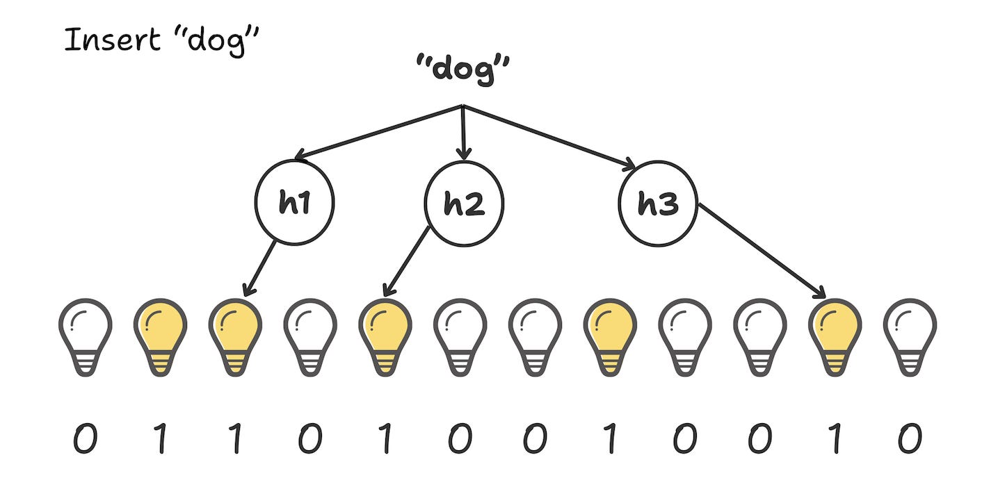
Current State: Switches 1, 2, 4, 7, and 10 are now ON.
Act 3: The Dark room(fish)
Now, a query comes in for “fish”. Does fish exist? We hash “fish” and get the indices: 0, 4, and 8.
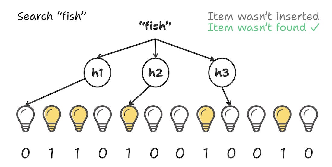
We check the array. Index 0 is off.
We stop.
There’s no need to check further. If “fish” were actually in the set, we would have flipped Switch 0 to ON. Since it is OFF, “Fish” is definitely not here.
Result: “Definitely No.”
Cost: Constant time (depends only on the time taken to hash the input through n hash functions), typically in nanoseconds on standard hardware. The work never increases, no matter how large the set becomes.
Act 4: The False Alarm (wolf)
Now, the villain arrives. A request comes in for “wolf”. We hash “wolf” and get indices: 1, 4, and 10.
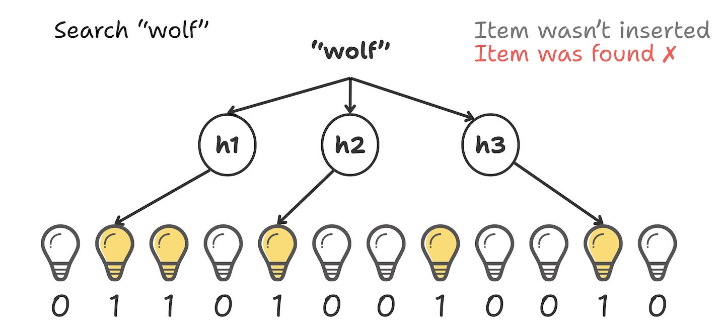
We check the array:
Switch 1 is ON (from Cat).
Switch 4 is ON (from Cat & Dog).
Switch 10 is ON (from Dog).
The Bloom Filter says: “Well, all the lights are on. So... yes? The wolf is probably here.”
But we never added wolf! The “wolf” just happened to land on the exact combination of bits turned on by Cat and Dog.
This is a False Positive. It is the price we pay for compression. The Bloom Filter says “Maybe,” so we have to check the database, only to find Wolf isn’t there.
Part 2: The Engineering Math (Managing the False Positives)
Now that we’ve seen how a “Wolf” can accidentally trigger a false positive, the natural question is: Can we fix it?
We can’t get rid of false positives completely, that’s the ‘tax’ we pay for using probabilistic data structures. If we wanted 100% accuracy, we’d have to use a standard HashMap and pay the heavy memory cost.
Our filter needs to be designed so that these “Wolf” moments happen rarely enough that they don’t crash our database. This is where we have to balance our inputs.
We can’t just pick a random array size or an arbitrary number of hash functions. If we guess wrong, the array fills up too fast, and suddenly everything starts looking like a “Maybe.” On the flip side, if we make it too large, we might be wasting too much RAM.
To get the math right, there are 4 things to consider :
n : The number of items to track.
p : The desired false positive rate (e.g., 0.01 for 1% error rate).
m : The total number of bits in the array needed (RAM cost).
k : The number of hash functions to run.
The probability of a false positive p is derived from the state of the bit array after n elements have been inserted using k hash functions. On doing some math, the optimal formula derived to determine the required number of bits m is:
And the optimal number of hash functions(k) is:
Let’s look at a quick example. Imagine you have 1 million keys and you’re okay with a 1% false positive rate (p = 0.01 and n is 1,000,000).
If you run those numbers:
m ≈ 9.6 million bits (≈ 1.2 MB of RAM)
k ≈ 7 hash functions
This is pretty wild, you are tracking a million items with high accuracy, and the whole thing fits into about 1.2 MB of memory. To put that in perspective, you’re protecting a database from millions of wasted hits using less memory than a single high res photo on your phone.
Part 3: The Project (Warden)
The concept and the math was there on the whiteboard, now we wanted to implement it and see if it actually holds up in a real system.
So, we built a small project called Warden. It’s essentially a lab experiment to simulate a specific distributed systems problem: Cache penetration.
Cache Penetration
Before looking at the code, let’s define the bug we’re trying to kill.
In a standard setup, you put a Cache (like Redis) in front of your Database to handle the load.
User asks for ID: 100. Redis finds it. Hit.
User asks for ID: 999 (doesn’t exist). Redis checks, finds nothing, and says Miss. You go to the database, search the disk, and find nothing.
Now, if an attacker requests 100 million random, non-existent IDs, Redis won’t help. Since they are all unique, they are all cache misses.
This means that every single request goes through the cache and hits your database, forcing it to check the disk just to say “No”. Your database CPU hits 100% doing unproductive work, which slows it down for everyone else, causing delays or downtime even for legitimate users.
The Experiment
To see if a Bloom Filter could stop this, I built a simple simulation with three parts:
The Storage Layer
A standard SQLite database seeded with 1 million user records.
(Note on Seeding: Inserting 1M rows individually is a massive bottleneck. By wrapping the inserts in a single Transaction, the seed time drops from minutes to about 6-7 seconds.)
The Middleware (The Shield)
This is the core logic of the system. A Go-based middleware sits directly in front of the database and maintains the Bloom Filter in memory.
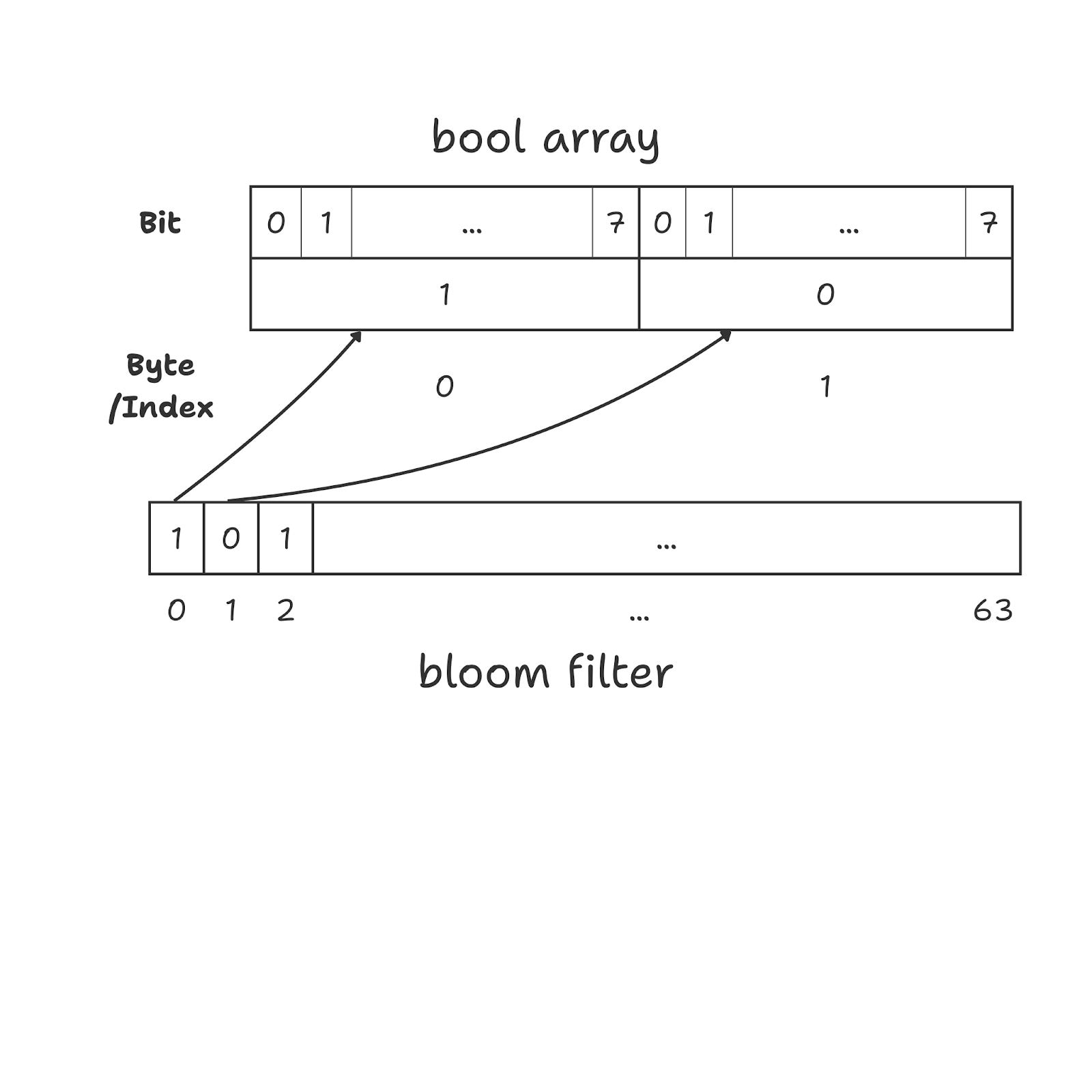
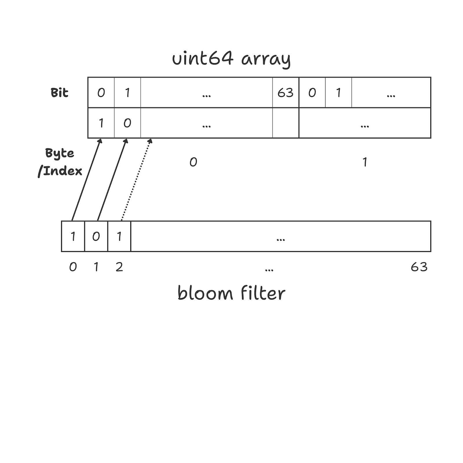
The filter is optimized using a uint64 array to keep the bit-packing as efficient as possible.
Normally, if we needed to store 1 million bits using a bool array, each bit would occupy an entire byte (8 bits). This means we would end up using roughly 1 MB of memory to store just 1 million bits.
By contrast, if we are using a uint64 array it allows us to pack bits efficiently. Each uint64 value stores exactly 64 bits in 8 bytes, so every bit is used with no wasted space. As a result, storing 1 million bits requires only about 125 KB of memory instead of 1 MB.
Only if the filter returns a “Maybe” does the request proceed to the database.
if !bloom.Contains(id) { return 404 }.
The Load Generator
To mimic a real-world attack, a custom load-testing script uses 100 concurrent workers to hammer the endpoint. The traffic is split 50/50 using a simple coin-flip logic:
Heads: Requests a valid user ID (Simulating normal traffic).
Tails: Requests a random, non-existent ID (Simulating a Cache Penetration attack).
Part 4: The Results
We ran the simulation on a local machine to see what would happen.
Run 1: Without the Filter
First, running it the standard way, letting every request hit the database. Since half the traffic was random junk, SQLite had to constantly check its index just to confirm those IDs didn’t exist.
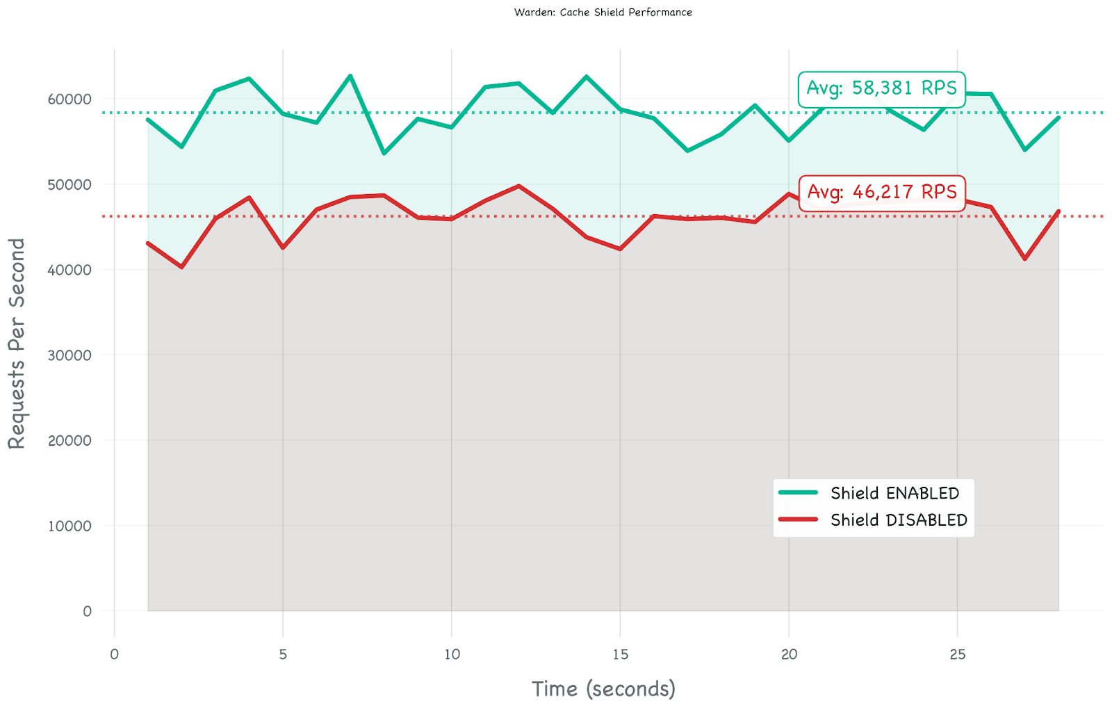
Result: ~46,000 requests/sec.
Observation: The CPU was working pretty hard just to handle the “Misses”.
Run 2: With the Filter
Then, on turning on the Bloom Filter middleware. The 50% “junk” traffic got caught in memory by our bit array. The database only had to deal with the valid requests.
Result: ~58,000 requests/sec.
We notice a 26% performance gain.
Testing for the “Worst Case”
A 50/50 split (half real users, half attackers) is pretty extreme and a stress test. On a normal Tuesday, it’s probably just 99% valid traffic.
So why even bother testing for a scenario like that?
A good analogy to understand this is a seatbelt. A seatbelt isn’t worn because a crash is expected on every trip, it’s worn so that when things go sideways, the protection is there.
On a good day: The Bloom Filter is just a tiny, static slice of RAM. It stays silent in the background, the overhead is negligible.
On a bad day: Maybe a scraper hits our endpoint, or bots try to brute-force a login. Suddenly, that “junk” traffic spikes to 50% or more. Bloom filter becomes the only thing between our db and downtime.
The Verdict
The stress test showed a 26% performance boost.
Half the traffic was filtered before it ever touched the disk. It’s a simple trade-off: spending a tiny bit of cheap memory to protect the most expensive part of the stack.
Final Thoughts
Probabilistic data structures like Bloom Filters feel like magic because they break the traditional rules of storage.
They accept a world where “Maybe” is a valid answer, and in doing so, they unlock performance that exact structures just can’t match.
Warden was a fun way to prove that you don’t need a massive infrastructure budget to build a resilient system, you just need a few million bits and the right math.
Code : https://github.com/eventuallyconsistentwrites/warden